Chaos Vis: Generate Art From Chaotic Systems

Recently, my Instagram reels on @bo_is_coding managed to reach over 100,000 accounts. As a result, I thought I might write a blog post to share more about the project.

@bo_is_coding

Chaotic system visual works

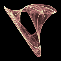
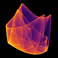
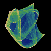
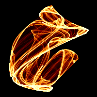
Math. Programming. Art. Sharing cool things I love, hoping you'll love them even more :)

Open Instagram profile

This blog aims to explain the project in two parts:

The code part (What did I do? How to optimize it?)
The math part (What did I create? What exactly are these images?)

The Code Part

A bit of Origin Story

Before we start diving into the logic, I would like to start with some background: I originally encountered the concept of chaotic systems in my ODE class in University, then I ran into this Random Attractors blog post by Paul Bourke.

I fell in love with these unique visuals immediately. Beginning with the Python and C implementations provided in the blog, I refined the code and expanded it into a fuller pipeline with improved performance and added functionality.

I am deeply grateful to Paul Bourke. Without his original work and inspiration, this project would never have come to life.

The core logic mentioned in his blog post is fairly simple:

Choose 12 random numbers $a_0,b_0$ through $a_5,b_5$ to initialize a quadratic map.

x_{n+1} = a_0 + a_1 x_n + a_2 x_n^2 + a_3 x_n y_n + a_4 y_n + a_5 y_n^2

y_{n+1} = b_0 + b_1 x_n + b_2 x_n^2 + b_3 x_n y_n + b_4 y_n + b_5 y_n^2

Choose 2 more random numbers $x_0,y_0$ as the starting position.
Starting from $x_0,y_0$ $x_{0}, y_{0}$ , iterate the position several million times using the quadratic map and check if system is both bounded and chaotic
- "bounded" should be self-explanatory. We want to ensure the system does not just shoots away indefinitely. If the point just shoots away from the center, several billion iterations would usually result in a line, a curve, or some extremely sparse pattern that is hard to visualize.
- "chaotic" means points that are really close to each other end up further away from each other as simulation goes on. In other words, we have the butterfly effect. Tiny differences in intitial condition are magnified my the simulation and results in huge divergences later in time (Paul Bourke's blog covers this part in-depth).
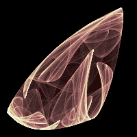
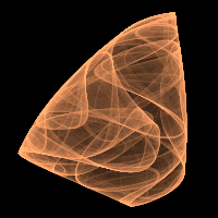
Finally, we can plot a heat map to visualize where the points have been landing during the simulation, and some of them look great!

Good Heat Maps, Bad Heat Maps

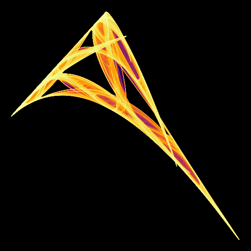
This all looks pretty good, but when I first tried out my local implementation, some of the resulting heat maps didn't look particularly interesting. Here is one such example:

This is pretty much just a line...

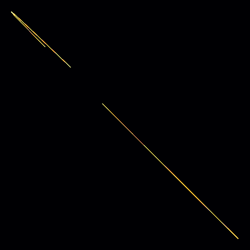
I usually have to sit in front of the computer and generate tens of random attractors to get a single descent looking heat map. While I found the process similar to the slot machine and somewhat addictive at times, I wanted to find a solution that can automatically filter for interesting heat maps.

My original plan, as most people might guess, was to incorporate AI and train a Convolutional Neural Network of some sort. As I was preparing my training data folder, however, I accidentally sorted all images by their size:

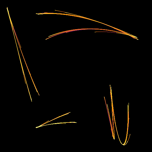
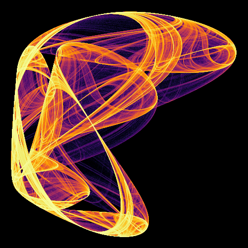
I immediately noticed a pattern: The bigger an image is, the better it looks!

This makes sense from an information theory perspective. Modern image formats are really efficient compressors, thus the image file size serves as an approximation of how much information an image contains. The more information an image contains, the more likely it is to look complex and interesting.

If we save the heat map plotted from the first several million iterations, we can look at its file size to programmatically determine how pretty the final heat map would be. It's not a perfect metric and I manually discover beautiful small "hidden gems" every now and then, but it's a very useful filter to have.

Accelerating Python with JIT

Another issue I wanted to solve was the unbearably slow speed of Python.

The simplest solution is to just use C/C++/Rust/Zig or some other faster language from the very beginning, eliminating the speed issue at its very root. However, I've been spoiled by the convenience of Jupyter Notebooks, particularly for this type of experimental projects.

While there are fabulous repos like xeus-cling that enables running faster languages on Jupyter Notebooks, by the time I found out its existence I already wrote too much Python code, and the switching cost was simply too high.

Luckily, there are ways to make Python faster. One useful tool is Numba, a Just In Time (JIT) compiler for Python. For numerical Python functions, Numba compiles it into machine code on first execution. Later calls to the function then invoke the compiled machine code, which is a lot faster than raw Python.

I took some time to benchmark the performance between naive Python, Numba accelerated Python, and C. I implemented the same dynamical system simulation code in three different ways, asking it to render 10000 attractors for up to a certain number of iterations (from 1000 to 1,000,000) and determine whether they are chaotic attractors.

Following is the chart. The time taken is the Y axis, and the number of iterations is the X axis, note both axes are logarithmic. On larger displays, you may click on the legend to toggle individual series, and use the top right buttons to zoom in / out of the chart.

Loading chart...

Here is the Colab Notebook I used to produce the benchmark data.

In general, C provides a 200x-300x speedup over naive Python. Numba JIT is one order of magnitude slower than C, but still provides an impressive 10-20x speedup over naive Python - fast enough for my use case.

The Math Part

Originally this section of the blog was supposed to be condensed into a single sentence near the start - a sentence that concisely describes what exactly these generated images are in mathematical terms. However, the deeper I went into the rabbit hole, the more I realized I actually didn't know what these images are, and their nature was much more complex than I expected.

Attractors? Trajectories!

At first glance, a good description of these images would be something like "A heatmap visualizing random attractors". The name carries over quite nicely from the original blog by Paul Borke.

However, that is not fully accurate. To properly understand these images, we need to first understand what an attractor is.

One common definition of an attractor is a type of structure in a dynamical system. Think of a dynamical system as something whose state changes over time (e.g. weather, a swinging pendulum, a population size, etc.). It can be visualized as a point moving around in a space of possibilities.

An attractor is a region or shape in the space that the point gets drawn toward. In more formal terms, an attractor is a set $A$ in the state space $X$ such that:

$A$ is invariant: Trajectories starting in $A$ remain in $A$ .
$A$ is attracting: There exists some neighborhood $U$ of $A$ such that for every initial condition $x_0 \in U$ we have:

\operatorname{dist}(\phi_t(x_0), A) \to 0 \quad \text{as } t \to \infty

In more simple terms:

Whatever starts in $A$ stays in $A$ forever.
There's some neighborhood $U$ around $A$ . Whatever starts in $U$ eventually gets really close to $A$ .

Using weather as an example, let the temperature be $T$ . If we set the attractor to just be a point $A = \{T=5\}$ , we are essentially asserting that the temperature approaches $5$ degrees in the long run.

In this sense, attractors can be seen as "stable substates" in the dynamical system that traps any traffic flowing into it.

Note multiple attractors with different basins of attraction can exist at the same time in a dynamical system. Back to the temperature example, we can have any temperature above 50 degrees approaching 100 degrees, and anything 50 degrees or below approaching 0 degrees. Now we have two attractors, one with $U = \{T\leq 50\},\ A=\{T=0\}$ , another with $U = \{T>50\},\ A=\{T=100\}$

It is very difficult to verify two sets make up an attractor purely through simulation. One way is to randomly sample points from the basin of attraction and iterate on them. Given enough iterations, all points should asymptotically approach the attractor. Additionally, any points already in the attractor remain in it, as the attractor is invariant. Although this still can't really determine the attractor for certain like a proof, this is as close as we can get solely through numerical computation, and if the number is big enough it can be considered strong evidence.

However, we're not really doing any of that! We're just picking a single random starting point and iterating on it many times. As a result, we are not working with an attractor; we are only working with one singular trajectory.

Now mathematicians aren't too interested in specific trajectories. Usually they're more concerned with the properties or characteristics of the entire system, or large abstract substates of the system, as it gives them theoretical tools to do cool proofs. Specific numerical trajectories are usually not the first citizen in math literature.

Once we pick the trajectory and iterate it for several mini iterations, we can compute the Lyapunov exponent to determine whether the system is chaotic. This sounds fancy, but really we're just sampling points that are really close to each other, as we evolve the system, check if points close to each other get further apart or converge closer to each other? If points become further apart, the Lyapunov exponent is positive. If the points become closer together, then the Lyapunov exponent is negative.

The idea is that if points grow closer over time, the system is most likely to settle into something stable, either some fixed point or a fixed cycle, and the resulting pattern is usually not that interesting. If the points grow further apart from each other, however, it exhibits chaotic behavior and tends to never repeat itself. The key insight here is that if points that are really close to each other eventually grow far apart, any small perturbation of the initial condition grows larger over time. We essentially have the butterfly effect, where even the smallest changes result in completely different trajectories.

Of course, we also check for other important properties like boundedness. If points shoot out really quickly, we don't bother tracing it. We only look for ones that are both chaotic and also stay bounded within a certain region, because then if we plot the points' landing position as a heat map, we are more likely to get something that is visually pleasing.

This is the first filter.

However, it's important for us to understand what can go wrong here. When we are running the simulation, we don't have infinite precision; instead, we are using floating-point numbers, particularly if we are using doubles. The accuracy is $2^{-1074}$ in the best possible sceneario, but for normal doubles the accuracy is somewhere near $2^{-52}$ .

So now you see the issue. If we are working with a chaotic system for millions of iterations and we are cropping, we're truncating the number every single iteration. After enough iterations, the truncation error grows larger, and we are essentially working with something that is nothing like the original trajectory.

As a result, we never rigorously prove the Lyapunov exponent. This is at best a numerical simulation that is not guaranteed to be perfect.

Once we have it passing all the tests, then we create the actual thing, the actual image and videos, by repeating the iteration billions of times. This is really where things start to bother me, because you see, the floating-point number issue only grows bigger and bigger. I'm pretty confident that even if it's an extremely small truncation error, eventually it grows to the point, after 10 billion iterations, probably throws the entire trajectory off. In this sense, we are never capable of producing an authentic chaotic trajectory.

This brings us to another point: the idea of a chaotic pattern is usually such that the system can never repeat itself. However, in this case there are only a finite number of states. In a 2D system, we only have 2^64 possible floating-point numbers, and the total number of states is thus 2^64 times 2^64, which is equal to 2 to the power of 128 possible states. In actual life, in our simulation, after we complete 2 to the power of 65 iterations, in the next iteration the system simply has to repeat itself.

At this point, our entire perception shifts. This is not really a chaotic system anymore due to the finite number of states and the lack of infinite precision. We are bound to repeat ourselves, and we can't quite simulate perfect chaos.

In finite precision, the computation is really a deterministic dynamical system on a finite state space. That means every orbit must eventually fall into a periodic cycle. If one wants a genuinely probabilistic coarse-grained model, a better candidate would be a transition matrix between pixels or bins.

In fact, if we look at all the possible states, we basically have a Markov chain, a trivial Markov chain too, since each state deterministically, 100%, results in the next state.

Now the picture that we're creating is essentially: we are simulating the first 10 billion or less iterations, and we're automatically zooming in on those iterations on an appropriate rectangle that contains the entire trajectory. Then we're seeing whether the heatmap, which we're trying to plot, is basically where the system landed (the states the system landed in) and plot a heatmap. Note here that we're not plotting the heatmap. We have really two layers of abstractions here:

The original floating-point numbers. There is a lower since there is a cutoff in both the x and y axes. There are only a finite number of floating-point numbers between the limits, and thus we have a conceptual. This provides a higher granularity and it's faithful to the simulation.
Alternatively, we usually don't have a pixel for every possible floating-point number, because that's a huge waste. Also, floating-point numbers are not distributed evenly. Instead, we usually use pixels to divide up the limits into smaller rectangles and see smaller rectangles to save memory. As a result, here we are applying convolution on the original image, where, based on the floating-point distribution, the convolution kernel actually auto-resizes to some extent.

In this sense, it will be interesting, and it is on my plan to create an actual Markov chain where the transition probability from pixel A to pixel B is simply the number of states in pixel A that result in a transition to pixel B. Now we are actually probabilistic; however, that's not currently implemented in the project.

So now you see the nature of this simulation and how it's difficult to accurately use mathematics to give it an accurate description. It's tempting to say it's related to an attractor, but we know very little about the dynamical system and the attractors in it, as we are only looking at a single "trajectory" in the system. At the same time, it's not even a faithful trajectory due to the truncation we apply due to the finite accuracy of floating point numbers and the truncation we apply at each step of the simulation. We know for a fact the trajectory will intercept itself, will repeat itself, unlike an authentic chaotic trajectory. And the more chaotic the trajectory is, the less accurate is our numerical simulation. Finally, we can't even make any claims on whether the trajectory is chaotic, since we can only give an approximation of the Lyapunov exponent.

And ultimately, when we reduce it down to an image, it's not even an exact convolution, since each pixel has the same side lengths, but the floating-point numbers are not evenly distributed. It's not guaranteed to equally distribute across the pixels within the image.

based on that, the best I can say is something like:

The figure is a finite-resolution visualization of the empirical visit distribution of a long floating-point pseudo-orbit generated by a randomly sampled quadratic planar map from a single initial condition, retained only when the sampled orbit remains bounded and exhibits a positive finite-time Lyapunov estimate.